Tutorial: Single chromosome optimization using OpenMiChroM
This tutorial performs optimization in the MiChroM Parameters (Second-order optimization -> Hessian inversion)
The first step is to import the OpenMiChroM modules.
To install OpenMM and OpenMiChroM, follow the instalation guide.
The inputs and apps used in this tutorial can be downloaded here.
Types optimization is available starting in the OpenMichroM version 1.0.7.
[1]:
# OpenMiChroM simulation module
from OpenMiChroM.ChromDynamics import MiChroM
# Optimization of MiChroM parameters module
from OpenMiChroM.Optimization import CustomMiChroMTraining
# Analysis tools module
from OpenMiChroM.CndbTools import cndbTools

# Extra modules to load and plot .dense file
import matplotlib.pyplot as plt
import matplotlib as mpl
from sklearn.preprocessing import normalize
import numpy as np
import pandas as pd
import h5py
from scipy.optimize import curve_fit
The second step is to have a look on the experimental Hi-C
A Hi-C file is required for the analysis and training of the MiChroM Potentials (Types and Ideal Chromosome). The file format chosen here is a matrix .txt file (we call it the dense file).
For this tutorial, we will use chromosome 10 from GM12878 in 100 kb resolution. To extract it from the .hic file, we can use juicer_tools with the folowing command. Please note that the juicer_tools java file is located at the apps folder located at the $HOME directory.
[2]:
%%bash
java -jar ~/apps/juicer_tools_1.22.01.jar dump observed Balanced -d https://hicfiles.s3.amazonaws.com/hiseq/gm12878/in-situ/combined.hic 10 10 BP 100000 input/chr10_100k.dense
WARNING: sun.reflect.Reflection.getCallerClass is not supported. This will impact performance.
WARN [2023-04-13T15:13:03,709]  [Globals.java:138] [main]  Development mode is enabled
INFO [2023-04-13T15:13:04,138]  [DirectoryManager.java:179] [main]  IGV Directory: /Users/ro21/igv
INFO [2023-04-13T15:13:04,317]  [HttpUtils.java:937] [main]  Range-byte request succeeded
This command downloads the .hic from the web and extracts the chromosome 10 in .dense format to the folder “input”.
You can get more information about it at the JuicerTools documentation.
Visualize the .dense file.
[3]:
filename = 'input/chr10_100k.dense'
hic_file = np.loadtxt(filename)

r=np.triu(hic_file, k=1)
r[np.isnan(r)]= 0.0
r = normalize(r, axis=1, norm='max')
rd = np.transpose(r)
r=r+rd + np.diag(np.ones(len(r)))
print("number of beads: ", len(r))
plt.matshow(r,norm=mpl.colors.LogNorm(vmin=0.0001, vmax=r.max()),cmap="Reds")
plt.colorbar()
number of beads: 1356
[3]:
<matplotlib.colorbar.Colorbar at 0x7faf98d94f70>
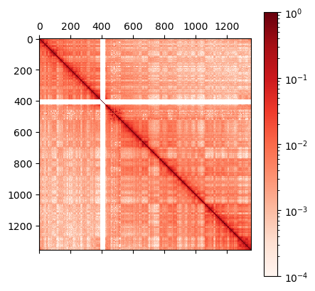
This Hi-C map has a resolution of 100 kb per bead, so the chromosome 10 model has a polymer chain with a total of 1356 beads.
The next step is to extract the sequence file containing the A/B compartments along the sequence by using the eigenvector decomposition.
Using the juicertools, you can extract the eigenvector file. The eigenvector has values both negatives and positives and here we will arbitrary set positives as B and negatives as A.
For more details about how it works, please take a look on this paper: https://pubs.acs.org/doi/full/10.1021/acs.jpcb.1c04174
[4]:
%%bash
java -jar ~/apps/juicer_tools_1.22.01.jar eigenvector -p Balanced https://hicfiles.s3.amazonaws.com/hiseq/gm12878/in-situ/combined.hic 10 BP 100000 input/chr10_100k.eigen
WARNING: sun.reflect.Reflection.getCallerClass is not supported. This will impact performance.
WARN [2023-04-13T15:13:12,055]  [Globals.java:138] [main]  Development mode is enabled
INFO [2023-04-13T15:13:12,506]  [DirectoryManager.java:179] [main]  IGV Directory: /Users/ro21/igv
INFO [2023-04-13T15:13:12,700]  [HttpUtils.java:937] [main]  Range-byte request succeeded
And visualize the .eigen file.
[5]:
eigen = np.loadtxt("input/chr10_100k.eigen")

index = np.arange(eigen.size)
df = pd.Series(eigen, index=index)

A1_df = pd.Series(np.zeros(eigen.size), index=index)
A1_df[df < 0] = df[df < 0]
B1_df = pd.Series(np.zeros(eigen.size), index=index)
B1_df[df > 0] = df[df > 0]

NA_df = df.isna()
# y = sc.signal.savgol_filter(A1,20, 2)

fig, axes = plt.subplots(ncols=1, nrows=2,
                         figsize=(6.4*3/2, 4.8*2/3),
                         gridspec_kw={'height_ratios': [1, 10]})
fig.tight_layout()

fig.subplots_adjust(hspace=0.05) # top=0.92, bottom=0.01, wspace=0.)

# sequence
A11_df = A1_df.copy()
A11_df[A1_df<0] = 1
B11_df = B1_df.copy()
B11_df[B1_df>0] = 1

axes[0].axis('off')
width=1
axes[0].bar(A11_df.index, A11_df,
       width,
       color="tab:red")
axes[0].bar(B11_df.index, B11_df,
       width,
       color="tab:blue")

axes[0].set_xlim([-50,eigen.size + 50])

# Eigen PC1
step=1
axes[1].fill_between(A1_df.index[::step], A1_df[::step],  0,
                facecolor="tab:red",
                alpha=0.8,
                label="A")
axes[1].fill_between(B1_df.index[::step], B1_df[::step],  0,
                facecolor="tab:blue",
                alpha=0.8,
                label="B")

axes[1].set_ylim([-0.05,0.05])
axes[1].set_xlim([-50,eigen.size + 50])

axes[1].set_ylabel('Eigen values, PC1')
axes[1].set_xlabel('Genomic distance (50 kb)')

axes[1].legend(title='compartments', bbox_to_anchor=(1.,1.45),
               frameon=False)

print("Number of beads: A1 = ", A1_df[A1_df<0].shape[0],
      ", B1 = ", B1_df[B1_df>0].shape[0])
Number of beads: A1 = 618 , B1 = 707

From the .eigen, file we can create the A/B sequence file.
[6]:
%%bash
awk '{if ($1 < 0) print "A1"; else print "B1"}' input/chr10_100k.eigen | cat -n > input/seq_chr10_100k.txt
echo "Number of beads: "
awk '{print $2}' input/seq_chr10_100k.txt | sort | uniq -c
Number of beads:
 618 A1
 738 B1
1# Types Interaction Opmization
In addition to the homopolimer term, MiChroM energy function has two main terms: the type-to-type and Ideal Chromosome interactions.
\({ U }_{\text{MiChroM} }(\vec { r } )={ U }_{ HP }\left( \vec { r } \right) +\sum _{\tiny{ \begin{matrix} k\ge l \\ k,l \in \text{Types} \end{matrix} } }{ { \alpha }_{ kl } } \sum _{\tiny{ \begin{matrix} i \in \{ \text{Loci of Type k}\} \\ j \in \{ \text{Loci of Type l} \} \end{matrix} }} f({ r }_{ ij }) + \sum _{ d=3 }^{ { d }_{ cutoff } }{ \gamma (d)\sum _{ i }{ f({ r }_{ i,i+d }) } }\)
In this section, the types interaction terms will be minimized.
The pipeline to perform the Types Potential Optimization is the following:
Run a long simulation using the homopolymer + customTypes potential of the
OpenMiChroMmodule. The first iteration can start with all parameters equal to zero or set to an initial guess.Get the frames from this simualtion to perform the inversion for Types.
In the end of the inversion, new values to types interactions will be produced.
Calcule the error/tolerance between the simulated and experimental parameters. If it is above the treshold, re-do steps 1-3 until reaching the treshold (usually 10% or 15% is enougth).
The Types file is a .txt with a matrix labeled with the values for each interaction. In this tutorial, we are training A and B types.
Lets create the initial file with this format:
A,B
0,0
0,0
For this matrix, we have AA AB BA BB interactions.
Save it as lambda_0
[7]:
%%bash
echo "A1,B1
0,0
0,0" > input/lambda_0

cat input/lambda_0
A1,B1
0,0
0,0
With all the required inputs, lets perform a simulation for iteration 0.
In MiChroM initiation there are some variables to setup:
time_step=0.01 (the time step using for integration, default is 0.01) temperature=1 (Set the temperature of your simulation) name=‘opt_chr10_100K’ (the simulation name)
[8]:
simulation = MiChroM(name='opt_chr10_100K', temperature=1.0, time_step=0.01)
    ***************************************************************************************
     **** **** *** *** *** *** *** *** OpenMiChroM-1.0.6 *** *** *** *** *** *** **** ****

         OpenMiChroM is a Python library for performing chromatin dynamics simulations.
                            OpenMiChroM uses the OpenMM Python API,
                employing the MiChroM (Minimal Chromatin Model) energy function.
      The chromatin dynamics simulations generate an ensemble of 3D chromosomal structures
      that are consistent with experimental Hi-C maps, also allows simulations of a single
                 or multiple chromosome chain using High-Performance Computing
                            in different platforms (GPUs and CPUs).
         OpenMiChroM documentation is available at https://open-michrom.readthedocs.io

         OpenMiChroM is described in: Oliveira Junior, A. B & Contessoto, V, G et. al.
      A Scalable Computational Approach for Simulating Complexes of Multiple Chromosomes.
                  Journal of Molecular Biology. doi:10.1016/j.jmb.2020.10.034.
                                              and
                                 Oliveira Junior, A. B. et al.
     Chromosome Modeling on Downsampled Hi-C Maps Enhances the Compartmentalization Signal.
                        J. Phys. Chem. B, doi:10.1021/acs.jpcb.1c04174.

                    Copyright (c) 2022, The OpenMiChroM development team at
                                        Rice University
    ***************************************************************************************
Now you need to setup the platform that you will use, the options are:
platform=“OpenCL” (it can also be CUDA or CPU depending of your system) GPU=“0” (optional) (if you have more than one GPU device, you can set the GPUs that you want [“0”, “1”,…,“n”])
[9]:
simulation.setup(platform="OpenCL")
Set the folder name where the output will be saved.
[10]:
simulation.saveFolder('iteration_0')
The next step is to setup your chromosome sequence and initial configuration.
[11]:
mychro = simulation.createSpringSpiral(ChromSeq="input/seq_chr10_100k.txt")
Load the initial structure in the simulation object.
[12]:
simulation.loadStructure(mychro, center=True)
Now it is time to include the force field in the simulation object
Lets separate forces in two sets:
Homopolymer Potentials
[13]:
simulation.addFENEBonds(kfb=30.0)
simulation.addAngles(ka=2.0)
simulation.addRepulsiveSoftCore(Ecut=4.0)
Chromosome Potentials
In this tutorial, it is used the CustomTypes potential. Here we need to pass a file that contains a matrix of interactions for each other different type of chromosome. To check that, you can look on the OpenMiChroM documentation.
[14]:
simulation.addCustomTypes(mu=3.22, rc = 1.78, TypesTable='input/lambda_0')
Note: these valeus for \(\mu\) and \(r_c\) were calculated for human GM12878 cells and can be changed for other species.
The last potential to be added is the spherical restraint in order to collapse the initial structure.
[15]:
simulation.addFlatBottomHarmonic(kr=5*10**-3, n_rad=8.0)
Now we will run a short simulation in order to get a collapsed structure.
There are two variables that control the chromosomes simulation steps:
block: The number of steps performed in each cycle. n_blocks: The number of blocks that will be perfomed.
In this example, to perfom the collapsing we will run \(1\times10^3 \times 10^2 = 1\times10^5\) steps
[16]:
block    = 1000
n_blocks = 100
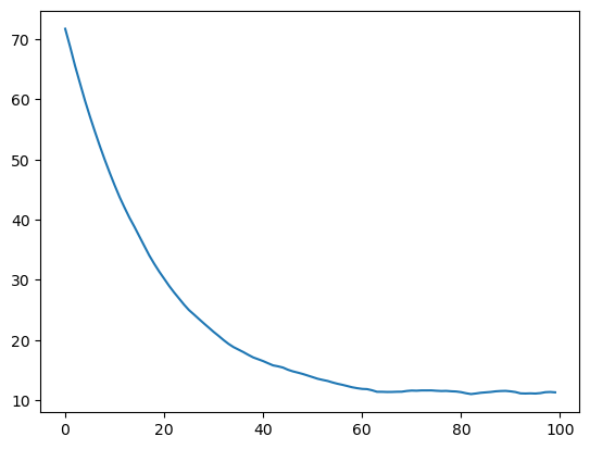
We can save the radius of gyration of each block to observe the convergence into the collapsed state (the time required here depends on the size of your chromosome).
[17]:
rg = []
[ ]:
for _ in range(n_blocks):
    simulation.runSimBlock(block, increment=False)
    rg.append(simulation.chromRG())

#save a collapsed structure in pdb format for inspection
simulation.saveStructure(mode = 'pdb')
Some details about the output for each block performed:
bl=0 is the number of each block, in this case we set increment=False, so the number of steps is not accounted. pos[1]=[X,Y,Z] the spatial position for the first bead. dr=1.85 show the average positions displacement in each block (in units os sigma). t=1000.0 ps the time step. in this case we set increment=False, so the number of steps is not accounted. kin=1.48 is the kinect energy of the system. pot=21.60 is the potential energy of the system. RG=11.809 is the radius of gyration in the end of each block. SPS=1538 is the steps per second of each block. A way to look how fast the computations are being performed. In this case, it was executed in a MB Pro 2021 with a Apple M1 Max.
Check the convergence of the radius of gyration:
[19]:
plt.plot(rg)
[19]:
[<matplotlib.lines.Line2D at 0x7fafa8dde040>]
The next step is to remove the restraint force in order to run the sampling simulation. It also adds a confinement potential with density = 0.1 (volume fraction).
[20]:
# Remove Flat initialized in Collapse
simulation.removeFlatBottomHarmonic()

# Add a confinement potential with density=0.1 (volume fraction)
simulation.addSphericalConfinementLJ()
[20]:
14.793027236438204
Initiate the optimization object for this tutorial section.
[21]:
optimization = CustomMiChroMTraining(ChromSeq="input/seq_chr10_100k.txt",
                                     TypesTable='input/lambda_0',
                                     mu=3.22, rc = 1.78)
The next step is to perform a long simulation to feed the optimization parameters.
In order to get a good inversion calcultation, it is important to have around \(1\times10^5\) frames from a certain amount of different replicas. For example, \(20\) replicas with \(5.000\) saved frames from each.
This can take some time, so in this tutorial we will use just 1 replica of \(5.000\) frames saved every \(1.000\) steps.
block = 1000
n_blocks = 5000
[ ]:
block    = 1000
n_blocks = 5000

for _ in range(n_blocks):
    # perform 1 block of simulation
    simulation.runSimBlock(block, increment=True)

    # feed the optimization with the last chromosome configuration
    optimization.prob_calculation_types(simulation.getPositions())
In the end of each replica simulation, we need to save some important values required to calculate the inversion.
We are saving these files using the H5 compression because it is faster to write/read.
Note: attention to this step. We have these 4 files for each replica for each iteration step. Be organized!
[23]:
replica="1"

with h5py.File(simulation.folder + "/Nframes_" + replica + ".h5", 'w') as hf:
    hf.create_dataset("Nframes",  data=optimization.Nframes)

with h5py.File(simulation.folder + "/Pold_" + replica + ".h5", 'w') as hf:
    hf.create_dataset("Pold",  data=optimization.Pold)

# Specific for Types minimization
with h5py.File(simulation.folder + "/Pold_type_" + replica + ".h5", 'w') as hf:
    hf.create_dataset("Pold_type",  data=optimization.Pold_type)

with h5py.File(simulation.folder + "/PiPj_type_" + replica + ".h5", 'w') as hf:
    hf.create_dataset("PiPj_type",  data=optimization.PiPj_type)
The first part of the optimization is finished. Look inside the output folder to see these 4 files that will be used in next step.
[24]:
%%bash
ls iteration_0/*.h5
iteration_0/Nframes_1.h5
iteration_0/PiPj_type_1.h5
iteration_0/Pold_1.h5
iteration_0/Pold_type_1.h5
The next part is the inversion. It is quite simple, just feed the optmization object with all replicas and make the inversion to get the new lambda file.
[25]:
inversion = CustomMiChroMTraining(ChromSeq="input/seq_chr10_100k.txt",
                                  TypesTable='input/lambda_0',
                                  mu=3.22, rc = 1.78)
[26]:
iterations = "iteration_0"
replica    = "1"

with h5py.File(iterations + "/Nframes_" + replica + ".h5", 'r') as hf:
    inversion.Nframes += hf['Nframes'][()]

with h5py.File(iterations + "/Pold_" + replica + ".h5", 'r') as hf:
    inversion.Pold += hf['Pold'][:]

# For Types
with h5py.File(iterations + "/Pold_type_" + replica + ".h5", 'r') as hf:
    inversion.Pold_type += hf['Pold_type'][:]

with h5py.File(iterations + "/PiPj_type_" + replica + ".h5", 'r') as hf:
    inversion.PiPj_type += hf['PiPj_type'][:]
With the parameters of all replicas, we calculate the inversion and get the new lambdas. It is calculated by using the Newton Method:
\(\lambda_1 = \lambda_0 - \delta\times\lambda_{actual}\)
\(\delta\) is the learning rate or damp, it can be adjusted in order to get values between [-1:0]. The average value of MiChroM’s parameters for Human GM12878 is -0.3 when generating \(1\times10^5\) configurations among different replicas.
[27]:
lambdas = inversion.get_lambdas_types(exp_map="input/chr10_100k.dense",
                                      damp=3e-7)

print(lambdas)
         A1        B1
0 -0.129980 -0.339399
1 -0.339399 -0.282689
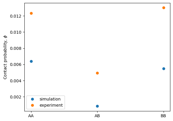
Save the new lambda (lambda_1) and other files to analyze the inversion.
[28]:
iteration = "0"
# Probabilities of As/Bs in the simulation and experiment
phi_sim = inversion.calc_phi_sim_types().ravel()
phi_exp = inversion.calc_phi_exp_types().ravel()
np.savetxt('iteration_0/phi_sim_' + iteration, phi_sim)
np.savetxt('iteration_0/phi_exp', phi_exp)
plt.plot(phi_sim[phi_sim>0], 'o', label="simulation")
plt.plot(phi_exp[phi_exp>0], 'o', label="experiment")
plt.ylabel(r'Contact probability, $\phi$')
labels_exp = ["AA", "AB", "BB"]
plt.xticks(np.arange(len(labels_exp)), labels_exp)
plt.legend()
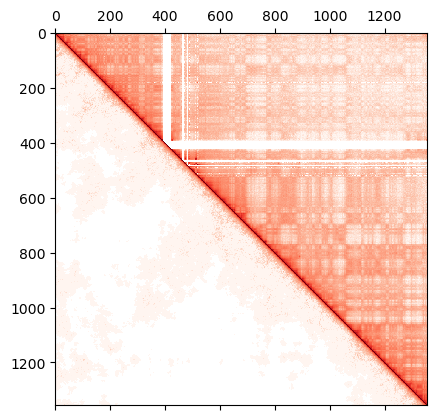
# Save and plot the simulated Hi-C
dense_sim = inversion.get_HiC_sim()
np.savetxt('iteration_0/hic_sim_' + iteration + '.dense', dense_sim)
dense_exp = np.loadtxt(filename)
dense_exp[np.isnan(dense_exp)] = 0.0
dense_exp = normalize(dense_exp, axis=1, norm='max')
r = np.zeros(dense_sim.size).reshape(dense_sim.shape)
r = np.triu(dense_exp, k=1) + np.tril(dense_sim, k=-1) + np.diag(np.ones(len(r)))
plt.matshow(r,
norm=mpl.colors.LogNorm(vmin=0.0001,
vmax=dense_sim.max()),
cmap="Reds")
# Save the new lambda file
lambdas.to_csv("iteration_0/lambda_1", index=False)
Redo these steps using the new lambda file (lambda_1) as input for Types potential in the next iteration.
The tolerance can be calculate using phi_sim_1 and phi_exp by the equation:
\(tolerance = \frac{|\phi_{sim}-\phi_{exp}|}{\phi_{exp}}\)
This is appended in to file tolerance_and_pearson_types.
[29]:
%%bash
cat tolerance_and_pearson_types
Tolerance: 0.621787 Pearson's Correlation: 0.854001
We included a folder named scripts that has some .py and .slurm files that can be used to run this optimization in parallel using slurm clusters. It is located in our github repository https://github.com/junioreif/OpenMiChroM.
2# Ideal Chromosome Interaction Opmization
Following the previous section protocoal, now it is time to learn how to minimize the Ideal Chromosome (IC) interaction, the last term of our hamiltonian
\({ U }_{\text{MiChroM} }(\vec { r } )={ U }_{ HP }\left( \vec { r } \right) +\sum _{\tiny{ \begin{matrix} k\ge l \\ k,l \in \text{Types} \end{matrix} } }{ { \alpha }_{ kl } } \sum _{\tiny{ \begin{matrix} i \in \{ \text{Loci of Type k}\} \\ j \in \{ \text{Loci of Type l} \} \end{matrix} }} f({ r }_{ ij }) + \sum _{ d=3 }^{ { d }_{ cutoff } }{ \gamma (d)\sum _{ i }{ f({ r }_{ i,i+d }) } }\)
The pipeline to perform the IC minimization is similar to the previous one:
Run a long simulation using the homopolymer + types potential + addCustomIC of the
OpenMiChroMmodule. The first iteration can start with all parameters equal to zero or set to an initial guess.Get the frames from this simualtion to perform the inversion.
In the end of the inversion, new values to the interactions will be produced.
Calcule the tolerance between the simulated and experimental parameters. If it is above the treshold, re-do steps 1-3 until reaching the treshold (usually 10% or 15% is enougth).
The IC file is a single column .txt with the values for each interaction. The file lenght should the genome distance (d) that you want to train. In the above equation, it goes from d = 3 to a certain cutoff that normaly would be 200 for the human chromosome.
Lets create the initial file with this format:
0
0
.
.
.
0
Save it as lambda_0.
[30]:
%%bash
rm input/lambda_0_IC &> /dev/null
for (( i=3; i<=1356; i++ )); do echo 0 >> input/lambda_IC_0; done
wc -l input/lambda_IC_0
2708 input/lambda_IC_0
Again, create the simulation that will colapse the initial structure.
[31]:
simulation_ic = MiChroM(name='opt_ic_chr10_100K', temperature=1.0, time_step=0.01)

simulation_ic.setup(platform="OpenCL")
simulation_ic.saveFolder('iteration_ic_0')
mychro_ic = simulation_ic.createSpringSpiral(ChromSeq="input/seq_chr10_100k.txt")
simulation_ic.loadStructure(mychro_ic, center=True)

# Adding Potentials section

# **Homopolymer Potentials**
simulation_ic.addFENEBonds(kfb=30.0)
simulation_ic.addAngles(ka=2.0)
simulation_ic.addRepulsiveSoftCore(Ecut=4.0)

# **Chromosome Potentials**
simulation_ic.addTypetoType()
simulation_ic.addCustomIC(IClist="input/lambda_IC_0",
                          dinit=3, dend=200)

# The restriction term for colapsing the beads
simulation_ic.addFlatBottomHarmonic(kr=5*10**-3, n_rad=8.0)
    ***************************************************************************************
     **** **** *** *** *** *** *** *** OpenMiChroM-1.0.6 *** *** *** *** *** *** **** ****

         OpenMiChroM is a Python library for performing chromatin dynamics simulations.
                            OpenMiChroM uses the OpenMM Python API,
                employing the MiChroM (Minimal Chromatin Model) energy function.
      The chromatin dynamics simulations generate an ensemble of 3D chromosomal structures
      that are consistent with experimental Hi-C maps, also allows simulations of a single
                 or multiple chromosome chain using High-Performance Computing
                            in different platforms (GPUs and CPUs).
         OpenMiChroM documentation is available at https://open-michrom.readthedocs.io

         OpenMiChroM is described in: Oliveira Junior, A. B & Contessoto, V, G et. al.
      A Scalable Computational Approach for Simulating Complexes of Multiple Chromosomes.
                  Journal of Molecular Biology. doi:10.1016/j.jmb.2020.10.034.
                                              and
                                 Oliveira Junior, A. B. et al.
     Chromosome Modeling on Downsampled Hi-C Maps Enhances the Compartmentalization Signal.
                        J. Phys. Chem. B, doi:10.1021/acs.jpcb.1c04174.

                    Copyright (c) 2022, The OpenMiChroM development team at
                                        Rice University
    ***************************************************************************************
Execute the simulation to colapse the initial structure
[ ]:
block    = 1000
n_blocks = 200

rg_ic = []

for _ in range(n_blocks):
    simulation_ic.runSimBlock(block, increment=False)
    rg_ic.append(simulation_ic.chromRG())

#save a collapsed structure in pdb format for inspection
simulation_ic.saveStructure(mode = 'pdb')

plt.plot(rg_ic)
It is time to remove the flat bottom constraint and include the spherical confinement mimicking the nuclear density.
[33]:
# Remove Flat initialized in Collapse
simulation_ic.removeFlatBottomHarmonic()

# Add a confinement potential with density=0.1 (volume fraction)
simulation_ic.addSphericalConfinementLJ()
[33]:
14.793027236438204
And create the IC optimization object.
[34]:
optimization_ic = CustomMiChroMTraining(ChromSeq="input/seq_chr10_100k.txt",
                                        TypesTable='input/lambda_0',
                                        IClist="input/lambda_IC_0",
                                        dinit=3, dend=200)
The next step is to perform a long simulation to feed the optimization parameters.
In order to get a good inversion calcultation, it is important to have around \(1\times10^5\) frames from a certain amount of different replicas. For example, \(20\) replicas with \(5.000\) saved frames from each.
This can take some time, so in this tutorial we will use just 1 replica.
[ ]:
block    = 1000
n_blocks = 5000

for _ in range(n_blocks):
    # perform 1 block of simulation
    simulation_ic.runSimBlock(block, increment=True)

    # feed the optimization with the last chromosome configuration
    optimization_ic.prob_calculation_IC(simulation_ic.getPositions())
It is time to save the important files required for the inversion.
These files are prefered to be saved using the H5 compression.
Note: attention to this step. We have these 4 files for each replica for each iteration step. Be organized!
[36]:
replica="1"

with h5py.File(simulation_ic.folder + "/Nframes_" + replica + ".h5", 'w') as hf:
    hf.create_dataset("Nframes",  data=optimization_ic.Nframes)

with h5py.File(simulation_ic.folder + "/Pold_" + replica + ".h5", 'w') as hf:
    hf.create_dataset("Pold",  data=optimization_ic.Pold)

# Specific for IC minimization
with h5py.File(simulation_ic.folder + "/PiPj_IC_" + replica + ".h5", 'w') as hf:
    hf.create_dataset("PiPj_IC",  data=optimization_ic.PiPj_IC)
[37]:
%%bash
ls iteration_ic_0/*.h5
iteration_ic_0/Nframes_1.h5
iteration_ic_0/PiPj_IC_1.h5
iteration_ic_0/Pold_1.h5
The next part is the inversion. We need to feed the optmization object with all replicas and make the inversion to get the new lambda file.
[38]:
inversion_ic = CustomMiChroMTraining(ChromSeq="input/seq_chr10_100k.txt",
                                     TypesTable='input/lambda_0',
                                     IClist="input/lambda_IC_0",
                                     dinit=3, dend=200)
[39]:
iterations = "iteration_ic_0"
replica    = "1"

with h5py.File(iterations + "/Nframes_" + replica + ".h5", 'r') as hf:
    inversion_ic.Nframes += hf['Nframes'][()]

with h5py.File(iterations + "/Pold_" + replica + ".h5", 'r') as hf:
    inversion_ic.Pold += hf['Pold'][:]

# For IC
with h5py.File(iterations + "/PiPj_IC_" + replica + ".h5", 'r') as hf:
    inversion_ic.PiPj_IC += hf['PiPj_IC'][:]
With the parameters of all replicas, we calculate the inversion and get the new lambdas. It is calculated by using the Newton Method:
\(\lambda_1 = \lambda_0 - \delta\times\lambda_{actual}\)
\(\delta\) is the learning rate or damp, it can be adjusted in order to get values between [-1:0]. The average value of MiChroM’s parameters for Human GM12878 is -0.3 when generating \(1\times10^5\) configurations among different replicas.
[40]:
lambdas_ic = inversion_ic.get_lambdas_IC(exp_map="input/chr10_100k.dense",
                                         damp=5e-4)

lambdas_ic.size, lambdas_ic[:5]
[40]:
(197, array([-0.06625294, -1.63630439, 0.2064909 , 0.12058404, -0.03533482]))
Save the new lambda (lambda_1_ic) and other files to analyze the inversion.
[41]:
iteration = "0"
# Probabilities of As/Bs in the simulation and experiment
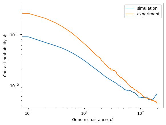
phi_sim = inversion_ic.calc_phi_sim_IC()
phi_exp = inversion_ic.calc_phi_exp_IC()
np.savetxt('iteration_ic_0/phi_sim_' + iteration, phi_sim)
np.savetxt('iteration_ic_0/phi_exp', phi_exp)
plt.plot(phi_sim, label="simulation")
plt.plot(phi_exp, label="experiment")
plt.ylabel(r'Contact probability, $\phi$')
plt.xlabel(r'Genomic distance, $d$')
plt.yscale('log')
plt.xscale('log')
plt.legend()
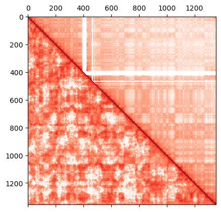
# Save and plot the simulated Hi-C
dense_sim = inversion_ic.get_HiC_sim()
np.savetxt('iteration_ic_0/hic_sim_' + iteration + '.dense', dense_sim)
dense_exp = np.loadtxt(filename)
dense_exp[np.isnan(dense_exp)] = 0.0
dense_exp = normalize(dense_exp, axis=1, norm='max')
r = np.zeros(dense_sim.size).reshape(dense_sim.shape)
r = np.triu(dense_exp, k=1) + np.tril(dense_sim, k=-1) + np.diag(np.ones(len(r)))
plt.matshow(r,
norm=mpl.colors.LogNorm(vmin=0.0001,
vmax=dense_sim.max()),
cmap="Reds")
# Save the new lambda file
np.savetxt("iteration_ic_0/lambda_1", lambdas_ic)
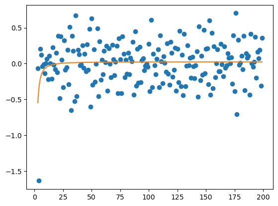
The simulated interaction terms (lambdas_1 data) can be used to fit a model in order to run production simulations with longer cutoffs in the IC energy term. The resulting model is used in the addCustomIC method of the OpenMiChroM class.
[43]:
def objective1(x, a, b, c):
    return -a / np.log(x) - b / x**2 - c / x

y = lambdas_ic
x = np.arange(3, lambdas_ic.size + 3)
plt.scatter(x, y, label='simulation')

# curve fit
popt, pcov = curve_fit(objective1, x, y)
a, b, c = popt
standard_dev = np.sqrt(np.diag(pcov))

# IC generated model
print(popt, standard_dev)

# plot the fit
x_fit = x
y_fit = objective1(x_fit, a, b, c)

plt.plot(x_fit, y_fit, label='fitting',
             color='#ff7f0e')
[-0.14260129 3.58641988 0.82703462] [0.15690074 5.51415182 1.68569841]
[43]:
[<matplotlib.lines.Line2D at 0x7faf889c9bb0>]
Nice job! You have completed the optimization tutorial of the MiChroM energy terms.