Temporally Correlated Active Noise Simulation Tutorial
Introduction
This tutorial is aimed at introducing nonequilibrium activity to OpenMiChroM simulations. First, we will go through a very brief introduction of the theoretical idea, then, the simulation procedures are discussed.
Theory
Activity, such as originating from molecular motors applying forces on the polymer, is modeled as an athermal drive experienced by each coarse-grained monomer. Since motors typically exhibit on/off dynamics, the athermal force is expected to be correlated in time, as opposed to the thermal noise that is temporally uncorrelated. To model activity, we add a novel noise-like term to the forces associated with a monomer, such that the equation of motion of the \(n\)-th monomer reads as follows:
where \(\gamma\) is the damping coefficient and \(U\) is the passive potential, like the harmonic bonds joining neighboring monomers in a polymer. \(\xi^{\rm therm}_n\) is the the thermal noise that is uncorrelated over time as well as across the chain:
The active noise kicks are given by \(f^{\rm act}(t)\), which are correlated over time and their correlation decays over a characteristic time scale \(\tau\):
The dynamics of the active force of the \(n\)-th monomer is governed by the following equation:
where \(\theta_a\equiv F^2\tau/\gamma\) is the active temperature-like quantity, and \(\eta(t)\) is a delta-correlated stationary Gaussian process.
Brownian Dynamics
Brownian dynamics only has forces and displacements, and no velocities. The positions after time \(\Delta t\), given by \(x(t+\Delta t)\) are computed based on the current forces \(h(t)\) and positions \(x(t)\).
where the last term is the thermal kick at temperature \(T\) with \(\mathcal{N}(0,1)\) representing a random Normal variable with zero mean and unit standard deviation. The net force experienced by the \(n\)-th monomer at time step \(t\) is given by \(h_n(t)\).
The net force for a monomer \(h(t)\), depends on the active force of the monomer \(f^{\rm act}(t)\), which is related to the active force in the previous time step \(f^{\rm act}(t-\Delta t)\). The active force on the \(n\)-th monomer at time \(t\) is obtained as follows:
where \(\mathcal{\tilde{N}}(0,1)\) is a random Normal variable that is different from the thermal one.
Next is a step-by-step guidance on how to setup and run OpenMiChroM simulations with correlated active noise. Users not familiar with running OpenMiChroM simulations, would greatly benefit from first going through the practice of running equilibrium OpenMiChroM simulations (see https://open-michrom.readthedocs.io/en/latest/Tutorials/Tutorial_Single_Chromosome.html). For users already familiar with OpenMiChroM, it is still the same simulation object that is created and basic steps of running the simulations are the same. The main differences are two fold: 1. Adding activity using a function addCorrelatedNoise(). One should make sure to add activity as the first force field. It is extremely important that the active force is assigned a force-group “0”. 2. Using a custom integrator ActiveBrownianIntegrator (see Integrator.py) that takes care of the active force which is hard-coded to be the force-group “0”. Hence the catutionary statement above.
Hope you follow along!
Simulations
Import modules
Active functions are
[ ]:
# revised to be compatible with OpenMiChroM 1.1.0 version
import sys
sys.path.append('../../')
import OpenMiChroM
from OpenMiChroM.ChromDynamics import MiChroM
from OpenMiChroM.Integrators import ActiveBrownianIntegrator
import numpy as np
Initialize simulation
[2]:
# Instantiate MiChroM object
sim = MiChroM(name='active_Rouse_sim', temperature=0.2, timeStep=0.001, collisionRate=1.0)

# specify platform and output destination
sim.setup(platform="cuda")
sim.saveFolder('./out')
active_correaltion_time = 5.0
#specify the integrator for correlated noise
#note that the force-group "0" is associated with the correlated active noise
sim.integrator = ActiveBrownianIntegrator(timestep=sim.timeStep, temperature=sim.temperature,
                                        collision_rate=sim.collisionRate, corr_time=active_correaltion_time)
    ***************************************************************************************
    **** **** *** *** *** *** *** *** OpenMiChroM-1.1.1rc *** *** *** *** *** *** **** ****

         OpenMiChroM is a Python library for performing chromatin dynamics simulations.
                            OpenMiChroM uses the OpenMM Python API,
                employing the MiChroM (Minimal Chromatin Model) energy function.
      The chromatin dynamics simulations generate an ensemble of 3D chromosomal structures
      that are consistent with experimental Hi-C maps, also allows simulations of a single
                 or multiple chromosome chain using High-Performance Computing
                            in different platforms (GPUs and CPUs).

         OpenMiChroM documentation is available at https://open-michrom.readthedocs.io

         OpenMiChroM is described in: Oliveira Junior, A. B & Contessoto, V, G et. al.
      A Scalable Computational Approach for Simulating Complexes of Multiple Chromosomes.
                  Journal of Molecular Biology. doi:10.1016/j.jmb.2020.10.034.
               We also thank the polychrom <https://github.com/open2c/polychrom>
                 where part of this code was inspired - 10.5281/zenodo.3579472.

                    Copyright (c) 2024, The OpenMiChroM development team at
                                        Rice University
    ***************************************************************************************
Using platform: CUDA
Load initial structure
[3]:
# generate a test sequence file of size n
n=10
with open('test_seq.txt','w') as seq_file:
    for ii in range(n):
        seq_file.write(f'{ii+1} A1\n')

# create a random configuration with the sequence file
init_struct = sim.createRandomWalk(ChromSeq='test_seq.txt')
sim.loadStructure(init_struct, center=True)

#uncomment below to save the loaded structure
#  sim.saveStructure(mode = 'auto')
Add forces
[4]:
# For the purpose of the simualtion we will consider a simple simulation of an active Rouse chain - harmonically bonded monomers with zero rest length
# the good things about active Rouse chain is that the dynamics may be calculated analytically and compared for verification.
# Any force-field available for OpenMiChroM, like self-avoidance, may be used.
# However, since Brownian Dynamics does not have momentum, it is prudent to make sure the time step is small enough for steep potentials.
# Using too large a time step with steep (or worse, diverging!) potentials will generate huge forces, possibly leading to explosion! wear your safety goggles!

# Now the force-fields(must be determined before sim.CreateSimulation()):
# first, add correlated noise.
# IMPORTANT: correlated noise should always be added as the *first* force-field.
# This is because force-group "0" is hard-coded as the active force within ActiveBrownianIntegrator
# act_seq contains the active force values F for each monomer. It needs to be the same size as the total number of monomers
# the values F_i in the list need not be the same, they can be heterogenous depicting varied motor activity
# below we consider a homogenously active polymer
F = 0.5
sim.addCorrelatedNoise(act_seq=F*np.ones(sim.N))

# add Harmonic bonds between monomers of the chain. Use sim.chains to get the number of chains.
# setting the rest length to zero since the analytical form is easier to calculate that way.
kb=5.0
sim.addHarmonicBonds(bondStiffness=kb, equilibriumDistance=0.0)

# adding soft-core self-avoidance
# repulsion is modeled using a sigmoid function with a finite overlap energy Ecut
# sim.addSelfAvoidance(Ecut=4.0, k_rep=20.0, r0=1.0)

# half-harmonic restraint as confinement
# sim.addFlatBottomHarmonic(kr=10.0, n_rad=20.0)
            ==================================
            Active Monomers (correlated noise) added.
            Active correlation time: 5.0
            Total number of active monomers: 10
            Total number of monomers: 10
            ==================================
Run intial collapse
[5]:
#run collapse simulation
sim.createSimulation()

sim.run(nsteps = 3000*10, report=True, totalSteps = 3000*10, checkSystem = False, interval=3000, blockSize = 3000)
# if repeate the code block, the simulation will extend, I'm not sure how to end it.
# save the collapsed structure -- uncomment below
# sim.saveStructure(filename='collapse',mode='ndb')
ActiveForce was added
HarmonicBond was added
Setting positions... loaded!
Setting velocities... loaded!
Context created!

Simulation name: active_Rouse_sim
Number of beads: 10, Number of chains: 1
Potential energy: 2.25000, Kinetic Energy: 0.56679 at temperature: 0.2

Potential energy per forceGroup:
                                 Values
ActiveForce              -2.980232e-08
HarmonicBond              2.250000e+01
Potential Energy (total)  2.250000e+01
#"Progress (%)" "Step"  "Speed (ns/day)"        "Time Remaining"
10.0%   3000    --      --
20.0%   6000    545     0:03
30.0%   9000    548     0:03
40.0%   12000   545     0:02
50.0%   15000   545     0:02
60.0%   18000   545     0:01
70.0%   21000   549     0:01
80.0%   24000   545     0:00
90.0%   27000   537     0:00
100.0%  30000   539     0:00
Run simulation
[6]:
# For the purpose of the tutorial we will just store the data in the xyz array for plotting
# you may instead save the data into cndb/ndb/pdb files and load into numpy arrays using cndbtools
# if you would like to save the data uncomment the lines below

# sim.initStorage(filename="active_Rouse_sim"") # initiate storage, however, this function has been deleted

xyz = [sim.getPositions()]

n_blocks = 500 # number of simulation blocks
block_size = 1000 # size of each block

for _ in range(int(n_blocks)):
    sim.run(nsteps = int(block_size),blockSize = int(block_size))
    # sim.saveStructure()
    xyz.append(sim.getPositions())

# sim.saveStructure(filename='lastframe',mode='ndb')
# sim.storage[0].close()

xyz = np.array(xyz)
print(xyz.shape) # the shape should be: (number of blocks, number of monos, deg. of freedom)
110.0%  33000   537     0:00
120.0%  36000   538     0:00
130.0%  39000   539     23:59:59
140.0%  42000   537     23:59:59
150.0%  45000   538     23:59:58
160.0%  48000   539     23:59:58
170.0%  51000   539     23:59:57
180.0%  54000   539     23:59:57
190.0%  57000   538     23:59:56
200.0%  60000   535     23:59:56
210.0%  63000   534     23:59:55
220.0%  66000   534     23:59:55
230.0%  69000   534     23:59:54
240.0%  72000   532     23:59:54
250.0%  75000   530     23:59:53
260.0%  78000   530     23:59:53
270.0%  81000   530     23:59:52
280.0%  84000   530     23:59:52
290.0%  87000   530     23:59:51
300.0%  90000   530     23:59:51
310.0%  93000   529     23:59:50
320.0%  96000   529     23:59:50
330.0%  99000   529     23:59:49
340.0%  102000  529     23:59:49
350.0%  105000  528     23:59:48
360.0%  108000  528     23:59:48
370.0%  111000  528     23:59:47
380.0%  114000  528     23:59:47
390.0%  117000  528     23:59:46
400.0%  120000  528     23:59:46
410.0%  123000  528     23:59:45
420.0%  126000  527     23:59:45
430.0%  129000  527     23:59:44
440.0%  132000  527     23:59:44
450.0%  135000  527     23:59:43
460.0%  138000  525     23:59:43
470.0%  141000  524     23:59:42
480.0%  144000  524     23:59:42
490.0%  147000  524     23:59:41
500.0%  150000  524     23:59:41
510.0%  153000  524     23:59:40
520.0%  156000  524     23:59:40
530.0%  159000  524     23:59:39
540.0%  162000  524     23:59:39
550.0%  165000  523     23:59:38
560.0%  168000  523     23:59:38
570.0%  171000  523     23:59:37
580.0%  174000  523     23:59:37
590.0%  177000  523     23:59:36
600.0%  180000  522     23:59:36
610.0%  183000  522     23:59:35
620.0%  186000  522     23:59:35
630.0%  189000  522     23:59:34
640.0%  192000  523     23:59:34
650.0%  195000  523     23:59:33
660.0%  198000  523     23:59:33
670.0%  201000  523     23:59:32
680.0%  204000  523     23:59:32
690.0%  207000  523     23:59:31
700.0%  210000  524     23:59:31
710.0%  213000  523     23:59:30
720.0%  216000  523     23:59:30
730.0%  219000  523     23:59:29
740.0%  222000  523     23:59:29
750.0%  225000  523     23:59:28
760.0%  228000  523     23:59:28
770.0%  231000  523     23:59:27
780.0%  234000  523     23:59:27
790.0%  237000  523     23:59:26
800.0%  240000  523     23:59:26
810.0%  243000  524     23:59:25
820.0%  246000  524     23:59:25
830.0%  249000  524     23:59:24
840.0%  252000  524     23:59:24
850.0%  255000  524     23:59:23
860.0%  258000  524     23:59:23
870.0%  261000  524     23:59:22
880.0%  264000  525     23:59:22
890.0%  267000  525     23:59:21
900.0%  270000  525     23:59:21
910.0%  273000  525     23:59:21
920.0%  276000  525     23:59:20
930.0%  279000  525     23:59:20
940.0%  282000  525     23:59:19
950.0%  285000  525     23:59:19
960.0%  288000  526     23:59:18
970.0%  291000  526     23:59:18
980.0%  294000  526     23:59:17
990.0%  297000  526     23:59:17
1000.0% 300000  526     23:59:16
1010.0% 303000  525     23:59:16
1020.0% 306000  526     23:59:15
1030.0% 309000  526     23:59:15
1040.0% 312000  526     23:59:14
1050.0% 315000  526     23:59:14
1060.0% 318000  526     23:59:13
1070.0% 321000  526     23:59:13
1080.0% 324000  526     23:59:12
1090.0% 327000  526     23:59:12
1100.0% 330000  526     23:59:11
1110.0% 333000  526     23:59:11
1120.0% 336000  526     23:59:10
1130.0% 339000  526     23:59:10
1140.0% 342000  525     23:59:09
1150.0% 345000  524     23:59:09
1160.0% 348000  525     23:59:08
1170.0% 351000  525     23:59:08
1180.0% 354000  525     23:59:07
1190.0% 357000  524     23:59:07
1200.0% 360000  524     23:59:06
1210.0% 363000  525     23:59:06
1220.0% 366000  525     23:59:05
1230.0% 369000  525     23:59:05
1240.0% 372000  525     23:59:04
1250.0% 375000  525     23:59:04
1260.0% 378000  524     23:59:03
1270.0% 381000  524     23:59:03
1280.0% 384000  524     23:59:02
1290.0% 387000  524     23:59:02
1300.0% 390000  524     23:59:01
1310.0% 393000  524     23:59:01
1320.0% 396000  524     23:59:00
1330.0% 399000  524     23:59:00
1340.0% 402000  524     23:58:59
1350.0% 405000  524     23:58:59
1360.0% 408000  524     23:58:58
1370.0% 411000  524     23:58:58
1380.0% 414000  524     23:58:57
1390.0% 417000  524     23:58:57
1400.0% 420000  524     23:58:56
1410.0% 423000  524     23:58:56
1420.0% 426000  524     23:58:55
1430.0% 429000  524     23:58:55
1440.0% 432000  524     23:58:54
1450.0% 435000  524     23:58:54
1460.0% 438000  524     23:58:53
1470.0% 441000  524     23:58:53
1480.0% 444000  524     23:58:52
1490.0% 447000  524     23:58:52
1500.0% 450000  523     23:58:51
1510.0% 453000  523     23:58:51
1520.0% 456000  524     23:58:50
1530.0% 459000  524     23:58:50
1540.0% 462000  523     23:58:49
1550.0% 465000  522     23:58:48
1560.0% 468000  519     23:58:48
1570.0% 471000  517     23:58:47
1580.0% 474000  513     23:58:46
1590.0% 477000  512     23:58:45
1600.0% 480000  511     23:58:44
1610.0% 483000  511     23:58:44
1620.0% 486000  510     23:58:43
1630.0% 489000  509     23:58:43
1640.0% 492000  508     23:58:42
1650.0% 495000  507     23:58:41
1660.0% 498000  507     23:58:41
1670.0% 501000  507     23:58:40
1680.0% 504000  507     23:58:40
1690.0% 507000  507     23:58:39
1700.0% 510000  507     23:58:39
1710.0% 513000  507     23:58:38
1720.0% 516000  507     23:58:38
1730.0% 519000  507     23:58:37
1740.0% 522000  507     23:58:37
1750.0% 525000  507     23:58:36
1760.0% 528000  508     23:58:36
(501, 10, 3)
Visualize trajectory
[7]:
#import the libraries for plotting
from matplotlib.animation import FuncAnimation
import matplotlib.pyplot as plt

# ipympl is necessary for dynamic plotting
# dynamic plotting is not supported inline
#%matplotlib ipympl

fig = plt.figure(1)
ax = fig.add_axes([0,0,1,1],projection='3d')

R0=sim.N**(0.5)

ax.scatter(xyz[0,:,0],xyz[0,:,1],xyz[0,:,2],'o',color='C0')
ax.plot(xyz[0,:,0],xyz[0,:,1],xyz[0,:,2],'-',color='C0')
ax.set_zlim(-R0, R0)
ax.set_xlim(-R0, R0)
ax.set_ylim(-R0, R0)

def update(ii):
    ax.cla()
    p=xyz[ii]
    ax.scatter(p[:,0],p[:,1],p[:,2],'o',color='C0')
    ax.plot(p[:,0],p[:,1],p[:,2],'-',color='C0')
    ax.set_zlim(-R0, R0)
    ax.set_xlim(-R0, R0)
    ax.set_ylim(-R0, R0)

anim = FuncAnimation(fig, update, frames=np.arange(1,400,1), interval=200, blit=False,repeat=False)

# uncomment below to save the animation
# anim.save('animation_active_sim.gif', writer='pillow')

plt.show()

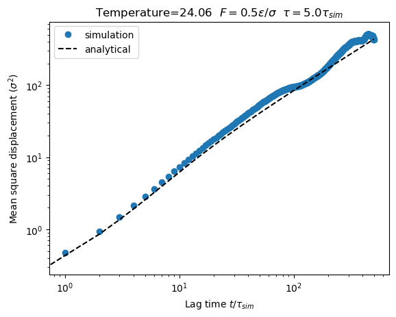
Verify dynamics
[8]:
from OpenMiChroM.CndbTools import cndbTools
cndbT = cndbTools()

def active_gas_MSD(t_lag, temp, F, tau, g, d=3):
    return d*(2*temp*t_lag/g + (2*F**2*tau/g**2)*(t_lag + tau*np.exp(-t_lag/tau)) - 2*F**2*tau**2/g**2)

def tau_rouse(p,kb,N,g):
    return g*N**2/(np.pi**2*kb*p**2)

def active_Rouse_MSD(t_lag, temp, F, tau, kb, N, g, d=3):

    rouse_modes=np.arange(1, N+1, 1)
    tau_mode_i=tau_rouse(rouse_modes, kb, N, g)
    val=(tau_mode_i*(temp+F**2*tau*tau_mode_i**2/(g*(tau_mode_i**2-tau**2)))*(1-np.exp(-t_lag/tau_mode_i))/(2*N*g)
        -(F*tau*tau_mode_i)**2*(1-np.exp(-t_lag/tau))/(2*N*g**2*(tau_mode_i**2-tau**2)))*0.5
    # print(val.shape)

    return (2*d*(temp+F**2*tau/g)*t_lag/(N*g) - 2*d*F**2*tau**2*(1-np.exp(-t_lag/tau))/(N*g**2) + 8*d*np.sum(val))
[9]:
# compute_MSD returns an (N * T) array with mononers in the first dimension and lag time in the second
msd_rouse = np.mean(cndbT.compute_MSD(xyz), axis=0)
[10]:
#%matplotlib inline

#lag times
ts = np.arange(0,xyz.shape[0], block_size*0.001)

plt.loglog(ts, msd_rouse,'o', label='simulation')
plt.loglog(ts, [active_Rouse_MSD(xx, sim.temperature*0.008314, F, sim.integrator.corrTime, kb, sim.N, 1.0) for xx in ts],'k--', label='analytical')
plt.legend()
plt.ylabel('Mean square displacement ($\\sigma^2$)')
plt.xlabel('Lag time $t/\\tau_{sim}$')
plt.title('Temperature={0:.2f}  $F={1:.1f}\\epsilon/\\sigma$  $\\tau={2:.1f} \\tau_{{sim}}$'.format(sim.temperature,F, sim.integrator.corrTime))
plt.ylim(msd_rouse[1]*0.5,max(msd_rouse)*1.5)
plt.show()
[ ]: